How the readiness score works

The question the app answers

Bhavitta answers two questions about a plan: will the money last to the end of the plan, and from what age could you stop working and still have it last. Everything on this page exists to make those two answers honest and reproducible. The engine is a single compiled Swift package that runs on your phone, on iOS natively and on Android through WebAssembly, so the same plan gives the same result on both.

1. Your plan is a timeline, not a form

A plan is a sequence of life stages from your current age to the end of the planning horizon. Each location stage has:

• A city and a lifestyle tier. Picking, say, Seattle at the Comfortable tier fills in an estimated annual living cost in today's US dollars and that city's typical local inflation rate. 49 curated cities are included; every estimate is editable and you can add your own city.
• Earned income and a blended tax rate for the years you work there. The tax rate is a single percentage applied to that stage's income. Bhavitta is not a tax calculator; it does not model brackets, slabs, or filing status.
• Household size, which scales the living cost.

On top of location stages you layer overlays: a home you own (mortgage, property tax, payoff age, sale with appreciation, selling cost and capital-gains rate), a property you rent out, a child's four years of college, a pension or Social Security (indexed guaranteed income from a start age), a recurring cost such as supporting parents, and one-time events such as a wedding, a windfall, or a down payment.

Years you leave uncovered do not break the model. An uncovered span after a location stage keeps that location and its living costs but drops earned income to zero: you still live there, you just no longer work there. Only a gap before your very first stage is filled with a generic mid-cost US baseline.

2. Every year, one cash-flow line

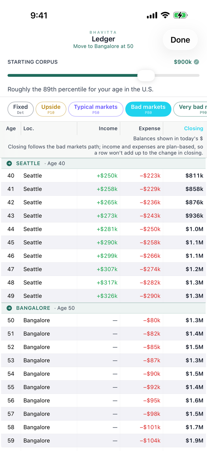
For each year of the plan the engine resolves the active stage and computes net cash flow: earned income minus tax, minus living expense, college, property and recurring costs, plus guaranteed income, rental income, home-sale proceeds and one-time credits. Then it rolls the balance forward:

Two deliberate choices sit in that recurrence. A plan that fails is allowed to go negative, so the ledger and chart show how deep the shortfall is instead of clamping at zero. And a deficit neither earns nor compounds; it is carried and can be paid back down by a later inflow such as a home sale or Social Security.

Indexing. Every amount you type is a today's-money figure. Income, living costs, guaranteed income and property tax grow with the active location's inflation rate from the start of the plan. Costs for an Indian city are stored in dollars and grow at India's inflation less the rupee-depreciation rate you set (defaults 6% and 3%, so about 2.9% a year in dollar terms). A separate display deflator converts any nominal balance back to today's money, switching rate the moment the active location changes, which is why a US-to-Bangalore plan reads sensibly in either basis.

3. Two ways to generate returns

Historical replay (the default)

The plan is run through every contiguous window of real market history. The embedded series is nominal annual total return on the S&P 500, price plus dividends, 1928 to 2023, from Aswath Damodaran's public dataset: 96 years, geometric mean about 9.8%, standard deviation about 19.5%. A 30-year plan therefore gets 67 trajectories, one starting in each of 1928, 1929, and so on; a 50-year plan gets 47. Nothing is randomised; it is deterministic, and it is the most faithful picture of what markets have actually done to a plan like yours, including the sequence-of-returns risk of retiring into 1929, 1966, or 2000.

A second source, Shiller real, deflates each year's return by US CPI so the plan runs in constant dollars with living costs held flat. The two are not comparable in dollar magnitude; use one or the other.

Monte Carlo

10,000 trials. Each year of each trial draws a return from a normal distribution with the expected return and volatility you set; the defaults are a deliberately conservative 7% and 12%. Draws are seeded from the plan itself, so the same plan always produces the same fan and the score does not jitter between opens.

4. What comes out

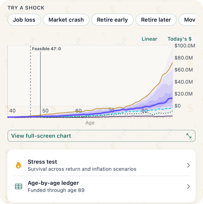
• A fan of balances. At every age the trials (or windows) are sorted and five lines are read off: P10, the optimistic upside only one in ten beats; P50, typical markets; P80, bad markets, the app's default benchmark; P90, very bad; P95, the worst case. Ten more quantile bands draw the probability cloud behind them.
• Survival rate. The share of trials in which the balance stayed above zero in every year of the plan, not just the last one. A path that is broke for twenty years and then rescued by a house sale does not count as surviving.
• A year-by-year ledger for any percentile path: opening balance, income, tax, each expense line, market gain and closing balance, in today's money by default.

5. The readiness score

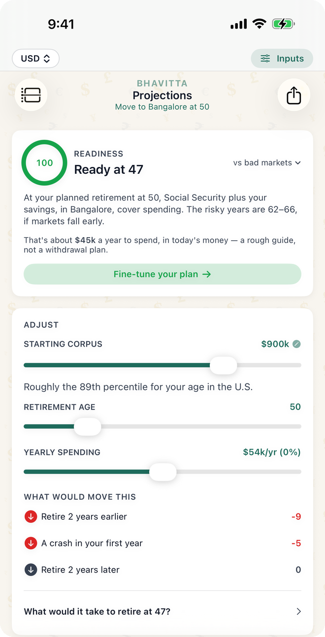
The 0 to 100 score combines the survival rate with a cushion test at your planned retirement age:

So survival alone can earn at most 80 points; the last 20 come from arriving at retirement with at least ten years of spending on the bad-markets line. A plan that survives on paper but starts retirement thin scores in the 80s, which is the point. The headline next to the gauge comes from a second computation, the earliest-retirement solver: it zeroes your earned income (and its tax) from a candidate age onward, leaving everything else in place, including where you live, your home, college and Social Security, and finds the earliest age at which survival still clears the benchmark. That age is the "Ready at 52" in the headline; if no age clears it, the headline says how far short the plan is at your own planned age. The sentence under it names the income sources that cover spending and the riskiest stretch of years on the bad-markets path.

6. Changing one thing

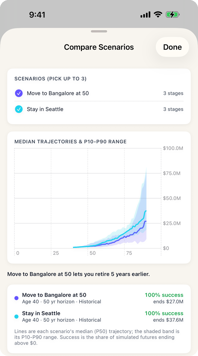
Three sliders under the score, starting corpus, retirement age and yearly spending, re-run the whole simulation on release and show the before and after. The what-if chips apply a named shock: a job loss (income gap), a market crash (a forced drawdown in a chosen year, applied identically to every trial and window), retiring earlier or later, a move abroad, a big expense. Compare overlays up to three scenarios and, with two selected, writes a one-line verdict such as "Moving to Bangalore at 50 lets you retire 4 years earlier", using retirement age first and survival rate as the tie-break.

The stress test is a five-by-five grid: expected return from two points below to two points above your baseline, inflation from one and a half points below to above, 200 trials per cell, coloured by survival. It shows which of the two assumptions your plan is actually sensitive to.

7. Spending shape

By default spending is constant real: flat in today's money, rising only with inflation. The optional Bernicke model eases real spending by 1.5% a year after 56 and levels off at 76, the "go-go, slow-go, no-go" pattern seen in retiree surveys. It usually raises survival; treat it as a view, not a promise.

8. What the model does not do

• No tax brackets, slabs, filing status, or treaty rules; one blended rate per stage, plus a capital-gains rate on property sales.
• No account types. EPF, NPS, PPF, 401(k) and IRA balances are simply part of the starting corpus; lock-ins, withdrawal limits and required minimum distributions are not modelled.
• One portfolio return. There is no asset allocation, bond ladder or glide path; the return you set, or history, applies to the whole balance.
• Historical replay uses US equity history for every plan, including plans lived in India.
• Healthcare, insurance and long-term care are not special; add them as a recurring cost or a one-time event if they matter to you.
• Display currency is a presentation conversion of dollar amounts; the rupee-depreciation input is the only currency-risk lever.

Defaults, in case you want to compare with your own spreadsheet: expected return 7%, volatility 12%, US inflation 3%, India inflation 6%, rupee depreciation 3%, Monte Carlo 10,000 trials, benchmark P80 at an 80% survival bar. All are editable in Inputs.